r-sf-make-grid-and-intersect
Make a grid and intersect points with the sf package
Francesco Bailo (francesco.bailo@sydney.edu.au)
Package for spatial analysis
library(sf)
## Linking to GEOS 3.11.0, GDAL 3.5.3, PROJ 9.1.0; sf_use_s2() is TRUE
Package’s documentation:https://cran.r-project.org/web/packages/sf/index.html
Other packages
library(tidyverse)
## ── Attaching packages ─────────────────────────────────────── tidyverse 1.3.2 ──
## ✔ ggplot2 3.4.0      ✔ purrr   1.0.1
## ✔ tibble  3.2.0      ✔ dplyr   1.0.10
## ✔ tidyr   1.2.1      ✔ stringr 1.5.0
## ✔ readr   2.1.3      ✔ forcats 0.5.2
## ── Conflicts ────────────────────────────────────────── tidyverse_conflicts() ──
## ✖ dplyr::filter() masks stats::filter()
## ✖ dplyr::lag()    masks stats::lag()
Read/Inspect shapefile
regions.sf <-
  sf::read_sf("data/Reg01012020_g_WGS84.shp")
st_crs(regions.sf)
## Coordinate Reference System:
##   User input: WGS 84 / UTM zone 32N
##   wkt:
## PROJCRS["WGS 84 / UTM zone 32N",
##     BASEGEOGCRS["WGS 84",
##         DATUM["World Geodetic System 1984",
##             ELLIPSOID["WGS 84",6378137,298.257223563,
##                 LENGTHUNIT["metre",1]]],
##         PRIMEM["Greenwich",0,
##             ANGLEUNIT["degree",0.0174532925199433]],
##         ID["EPSG",4326]],
##     CONVERSION["UTM zone 32N",
##         METHOD["Transverse Mercator",
##             ID["EPSG",9807]],
##         PARAMETER["Latitude of natural origin",0,
##             ANGLEUNIT["Degree",0.0174532925199433],
##             ID["EPSG",8801]],
##         PARAMETER["Longitude of natural origin",9,
##             ANGLEUNIT["Degree",0.0174532925199433],
##             ID["EPSG",8802]],
##         PARAMETER["Scale factor at natural origin",0.9996,
##             SCALEUNIT["unity",1],
##             ID["EPSG",8805]],
##         PARAMETER["False easting",500000,
##             LENGTHUNIT["metre",1],
##             ID["EPSG",8806]],
##         PARAMETER["False northing",0,
##             LENGTHUNIT["metre",1],
##             ID["EPSG",8807]]],
##     CS[Cartesian,2],
##         AXIS["(E)",east,
##             ORDER[1],
##             LENGTHUNIT["metre",1]],
##         AXIS["(N)",north,
##             ORDER[2],
##             LENGTHUNIT["metre",1]],
##     ID["EPSG",32632]]
The coordinate reference system is important as it defines the unit
(e.g. meters or degrees) for the grid size. In this case the CRS is
WGS 84 / UTM zone 32N or ID["EPSG",32632]] which is in meters (see
https://epsg.io/32632).
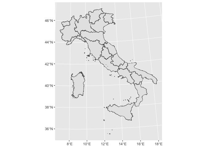
regions.sf %>%
  ggplot2::ggplot() +
  ggplot2::geom_sf()
Union
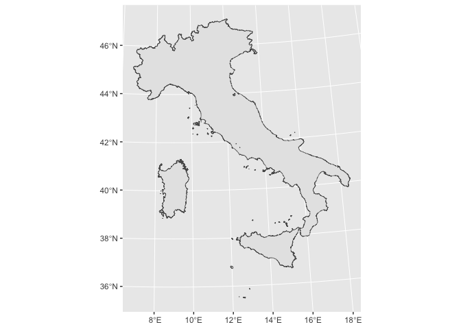
You want a mask to your grid, so if you gave multiple features (here 20 regions) you might want to combine them (resolving the internal boundaries). With sf and dplyr this can achieved with:
regions.sf$unit <-
  1

italy.sf <-
  regions.sf %>%
  dplyr::group_by(unit) %>%
  dplyr::summarize(AREA = sum(SHAPE_AREA))
italy.sf %>%
  ggplot2::ggplot() +
  ggplot2::geom_sf()
Making the grid
This is a two step process.
-
With
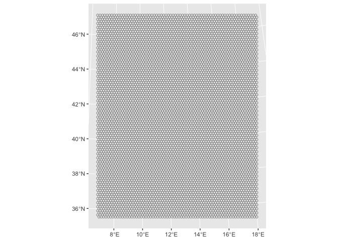
st_make_gridwe create the grid as simple feature object.cellsizeis in the unit of the mask feature (hereitaly.sfis in meters).square = FALSEcreates an hexagonal grid instead of a square grid. -
With
st_sfwe append to the simple feature object a data frame - for future data analysis.
italy_hex.sf <-
  sf::st_make_grid(italy.sf,
                   cellsize = 15000,
                   what = "polygons",
                   square = FALSE)
italy_hex.sf <-
  sf::st_sf(hex_id = 1:length(lengths(italy_hex.sf)),
            italy_hex.sf)
italy_hex.sf %>%
  ggplot2::ggplot() +
  ggplot2::geom_sf()
Cropping
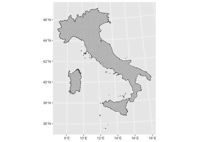
Finally we crop the grid
italy_hex_cropped.sf <-
  sf::st_intersection(italy_hex.sf,
                  italy.sf %>% st_make_valid())
## Warning: attribute variables are assumed to be spatially constant throughout
## all geometries
italy_hex_cropped.sf %>%
  ggplot2::ggplot() +
  ggplot2::geom_sf()
Intersecting with points
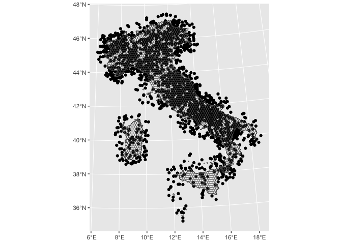
Let’s generate a buch of random points within the feature of
regions.sf. Note: we use st_buffer so that some points is going to
lay outside of the area we want to interst.
random_pnt.sf <-
  sf::st_sample(sf::st_buffer(regions.sf, 50000),
                size = rep(100, nrow(regions.sf)))
Our points are in the same CRS of all the other simple features (by design). If this is not the case, you must convert now to a common CRS with
random_pnt.sf <-
  sf::st_transform(random_pnt.sf, 32632)
and add a data frame to it
random_pnt.sf <-
  sf::st_sf(pnt_id = 1:length(lengths(random_pnt.sf)),
            random_pnt.sf)
random_pnt.sf %>%
  ggplot2::ggplot() +
  ggplot2::geom_sf() +
   ggplot2::geom_sf(data = italy_hex_cropped.sf, fill = NA, alpha = .2)
point_intersection.list <-
  sf::st_intersects(random_pnt.sf,
                    italy_hex_cropped.sf)
point_intersection.list
## Sparse geometry binary predicate list of length 2000, where the
## predicate was `intersects'
## first 10 elements:
##  1: 118
##  2: 59
##  3: (empty)
##  4: 76
##  5: 192
##  6: (empty)
##  7: (empty)
##  8: 282
##  9: 97
##  10: 415
Let’s make sure we don’t lose any point in the conversion from list to
vector in case they are out of the intersecting area (here the area of
italy_hex_cropped.sf). If they are, st_intersects intersect will
return a vector of length 0 instead of the index of the intersecting
feature. Vectors of length 0 in are lost like tears in the rain when we
unlist().
point_intersection.list[sapply(point_intersection.list, FUN = function(x) length(x) == 0)] <- NA
point_intersection.list
## Sparse geometry binary predicate list of length 2000, where the
## predicate was `intersects'
## first 10 elements:
##  1: 118
##  2: 59
##  3: NA
##  4: 76
##  5: 192
##  6: NA
##  7: NA
##  8: 282
##  9: 97
##  10: 415
Then we can add the resulting italy_hex_cropped.sf$hex_id to
random_pnt.sf.
random_pnt.sf$hex_id <-
  italy_hex_cropped.sf$hex_id[unlist(point_intersection.list)]
head(random_pnt.sf)
## Simple feature collection with 6 features and 2 fields
## Geometry type: POINT
## Dimension:     XY
## Bounding box:  xmin: 303389.3 ymin: 4930125 xmax: 451187.8 ymax: 5163356
## Projected CRS: WGS 84 / UTM zone 32N
##   pnt_id            random_pnt.sf hex_id
## 1      1 POINT (429070.5 4931973)    839
## 2      2   POINT (373757 5013787)    542
## 3      3 POINT (303389.3 4980196)     NA
## 4      4 POINT (388447.9 4930125)    639
## 5      5 POINT (451187.8 4989163)   1041
## 6      6 POINT (418223.4 5163356)     NA
random_pnt.sf %>%
  ggplot2::ggplot() +
  ggplot2::geom_sf(aes(colour = hex_id)) +
  scale_colour_viridis_c()
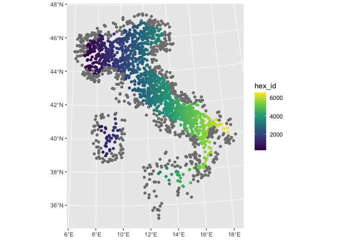
As we can see, hex_id is assigned from North West to South East.